In order to freeze a row in Excel, the following are the simple steps:
- Open your worksheet in Excel.
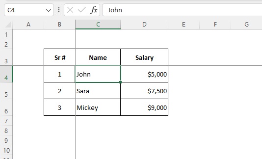
- Select the desired row you want to freeze, for instance, if you would like to free raw 3, then please select raw 4 or column C4 in this example.
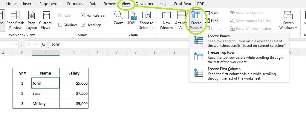
- Click on the “View” tab and then check “Freeze Panes”.
- Then select “Freeze Panes.” This option will freeze the desired chosen row and all above it.
- Under the frozen row, a horizontal line will appear, indicating that it has been frozen.